GeoScript at FOSS4G 2011

The GeoScript project has been quiet for a while now, but that does not mean developers haven't been busy. With the FOSS4G conference approaching development is ramping up. GeoScript will have a good showing this year, with two talks and one tutorial on the conference program.

The first talk, being delivered by Jared Erickson and myself, is titled GeoScript - Spatial Capabilities for Scripting Languages and will be an introduction of the project as a whole. The second talk titled Scripting GeoServer with GeoScript will be presented by Tim Schaub and myself and will focus in more on GeoScript as a scripting engine integrated with GeoServer.

The tutorial Working with GeoScript will be a 1.5 hour session and will provide a working introduction to GeoScript that will allow attendees to get their hands dirty with some code.

Developer turn out is going to be great this year. All four of David, Jared, Tim and myself will be attending this year so the four primary implementations will all be well represented. As well Ivan Willig is currently working hard on an implementation of GeoScript for Clojure that looks very interesting. Ivan hopes to get something up and on the site by FOSS4G.

Can't wait for the conference and look forward to seeing everyone there!

Styling with GeoScript

Over the past few months one of the major developments in GeoScript has been an API for styling. I finally got around to implementing the api for GeoScript python and am happy with how things are progressing.

GeoScript, being based on GeoTools, naturally uses SLD as the underlying styling engine. Those who have used SLD know that it is a complicated beast. While it is a very powerful symbology language, it is also very complex and verbose. And for those not familiar with SLD and XML it represents a substantial learning curve. GeoScript hopes to make SLD a bit more approachable.

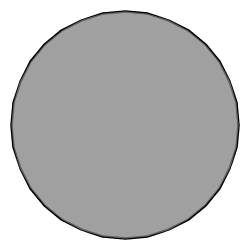
Let's start off with a simple example:

from geoscript.geom import *
from geoscript.style import *
from geoscript.render import draw

style = Stroke('black', 2) + Fill('gray', 0.75)
g = Point(0,0).buffer(0.2)

draw(g, style, (250,250))

Which results in:



The equivalent SLD for this style is:

<sld:UserStyle xmlns="http://www.opengis.net/sld" xmlns:sld="http://www.opengis.net/sld" xmlns:ogc="http://www.opengis.net/ogc">
<sld:FeatureTypeStyle>
<sld:Name>My Style</sld:Name>
<sld:Rule>
<sld:LineSymbolizer>
<sld:Stroke>
<sld:CssParameter name="stroke-width">2</sld:CssParameter>
</sld:Stroke>
</sld:LineSymbolizer>
<sld:PolygonSymbolizer>
<sld:Fill>
<sld:CssParameter name="fill-opacity">0.75</sld:CssParameter>
</sld:Fill>
</sld:PolygonSymbolizer>
</sld:Rule>
</sld:FeatureTypeStyle>
</sld:UserStyle>

Which is not all that bad as far as SLD goes. Let's look at a more complex example, one that anyone who as ever used GeoServer will be familiar with. The all too well known states layer that is styled with the popshade SLD. As far as SLD styles go popshade is actually relatively simple, but still involves hacking out about 100 lines of XML. What does the equivalent style look like with GeoScript?

style = Stroke()
style += Fill('#4DFF4D', 0.7).where('PERSONS < 2000000')
style += Fill('#FF4D4D', 0.7).where('PERSONS BETWEEN 2000000 AND 4000000')
style += Fill('#4D4DFF', 0.7).where('PERSONS > 4000000')
style += Label('STATE_ABBR').font('14 "Times New Roman"')

A bit more concise than the SLD equivalent. But for those who just can't go without their SLD remember that this is all geotools styling under the hood, so getting at the SLD is easy. So:

style.asSLD(sys.stdout)
style.asSLD('popshade.sld')

Dumps out the SLD that looks very similar to popshade.sld above.

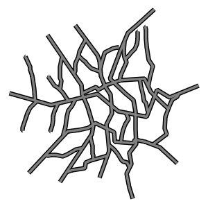
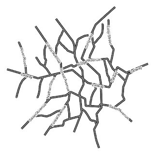
Continuing on with another example of a style type that is frequently used: line casing. More specifically rendering two lines on top of each other with the "bottom" line styled a few pixels thicker than the "top" line to give the appearance of a border or casing. This technique is commonly used to style road data.



First the SLD:

<FeatureTypeStyle>
<Rule>
<LineSymbolizer>
<Stroke>
<CSSParameter name="stroke">#000000</CSSParameter>
<CSSParameter name="stroke-width">5</CSSParameter>
</Stroke>
</LineSymbolizer>
</Rule>
</FeatureTypeStyle>
<FeatureTypeStyle>
<Rule>
<LineSymbolizer>
<Stroke>
<CSSParameter name="stroke">#ffffff</CSSParameter>
<CSSParameter name="stroke-width">3</CSSParameter>
</Stroke>
</LineSymbolizer>
</Rule>
</FeatureTypeStyle>

Not bad, but in GeoScript it is a one liner:

style = Stroke('#000000', 6) + Stroke('#ffffff', 3).zindex(1)

Let's add some labels to those lines:

style += Label('name', '12pt Arial').linear(follow=True,group=True,repeat=25).halo(Fill('#ffffff'), 2)

Those are just a few examples. Check out the api docs for a complete list of what is available. More to come soon so stay tuned.

Unwrapped JTS with Python

While Justin has been hard at work wrapping JTS and GeoTools in clear and simple Python syntax, I’ve been tinkering with some JTS classes that aren’t wrapped in GeoScript Python. Well, not wrapped yet. One of the great things about using Jython (or any scripting language written for the Java platform) is that you can still explore JTS and GeoTools even if some functionality isn’t implemented in GeoScript.

Jared produced a convex hull and minimum bounding circle with GeoScript Groovy in a recent post. I tried to replicate this workflow but quickly realized certain classes and functions weren’t available in GeoScript Python. Did it matter? Not very much in this case. Here’s the convex hull and minimum bounding circle for a shapefile of Washington weather stations produced in a previous post. Pay attention to what’s being imported.

from geoscript.layer import Shapefile
from geoscript.viewer import plot
from com.vividsolutions.jts.geom import GeometryCollection
from com.vividsolutions.jts.geom import GeometryFactory
from com.vividsolutions.jts.geom import PrecisionModel
from com.vividsolutions.jts.algorithm import MinimumBoundingCircle

#Get the point shapefile
staLayer = Shapefile('/home/gregcorradini/wa_stations.shp')

#Create a list of feature geometries
pntGeoms = [f.geom for f in staLayer.features()]

#Create a GeometryCollection from our list of points
geomColl = GeometryCollection(pntGeoms,GeometryFactory(PreciscionModel(),4326))

#Get the geometry collection's convex hull
geomConvexH = geomColl.convexHull()

#Get the geometry collection's minimum bounding circle
mCircle = (MinimumBoundingCircle(geomColl)).getCircle()

# Plot the geometries, BANG
plot(pntGeoms + [geomConvexH] + [mCircle])

I imported GeoScript modules and JTS Java classes in the example above. Jython can interoperate with Java libraries and classes because under the hood it’s Java. But how did I know what parameters a GeometryCollection accepted? I took a peek at the JTS Java doc and followed the bouncing argument ball. The weaving of colorful geometries happens after that thanks to the great plotting functionality from Justin.

There are tricks and trapdoors to this unwrapped exploration - the syntax is not as clean and intuitive as working with GeoScript Python. But a lot of magic still happens. I try to use functions that return geometry objects so I can plot them with the geoscript.viewer.plot function. This way I can see each step visually. Another advantage is that JTS and GeoTools have very well organized Java docs (here and there). It’s hard to fail at finding your way with road maps this good.

For example, mkgeomatics was deciding how to visually represent the output of a least-cost analysis he performed on a Bellingham, WA dataset. Part of the cartographic workflow used Voronoi diagrams that were built in ArcGIS. Both of us wondered if we could leverage GeoScript Python and JTS to solve the Voronoi diagram work. After a little sandbox scripting I came up with the following test code. It outlines how to derive a Voronoi diagram from a Delaunay triangulation (A more succinct way to build Voronoi diagrams would use the com.vividsolutions.jts.triangulate.VoronoiDiagramBuilder class. But Dr JTS produced an informative post on the relationship between both that I wanted to explore).

from geoscript.layer import Shapefile
from geoscript.viewer import plot
from com.vividsolutions.jts.geom import GeometryCollection
from com.vividsolutions.jts.geom import GeometryFactory
from com.vividsolutions.jts.geom import PrecisionModel
from com.vividsolutions.jts.algorithm import MinimumBoundingCircle
from com.vividsolutions.jts.triangulate import DelaunayTriangulationBuilder

#Get a point shapefile
staLayer = Shapefile('/home/gregcorradini/wa_stations.shp')

#Create a list of feature geometries
pntGeoms = [f.geom for f in staLayer.features()]

#Create a GeometryCollection from our list of points
geomColl = GeometryCollection(pntGeoms,GeometryFactory(PreciscionModel(),4326))

#Create a DelaunayTriangulationBuilder object and pass our geometry collection
dtb = DelaunayTriangulationBuilder()
dtb.setSites(geomColl)

#Get the Delaunay triangle faces
triangles = dtb.getTriangles(GeometryFactory(PrecisionModel(),4326))

#Make a pretty triangle picture
plot(pntGeoms + [triangles])

#Get the object's corresponding voronoi polygons in a java array
voronoiArray = dtb.getSubdivision().getVoronoiCellPolygons(GeometryFactory(PrecisionModel(),4326))

#Make a pretty picture
plot(pntGeoms + [i for i in voronoiArray])

That last Voronoi picture is hard to see in detail. So let's save off the Voronoi polygons to a shapefile and give each one the attributes of the original point that falls within it. The function 'changeGeometryType' is from a previous post.

#Create a voronoi geom.Poly schema based on old layer schema
voronoiSchema = changeGeometryType('voronoiWAStations',geom.Polygon,staLayer)

#Create voronoi layer
vLayer = ws.create(schema=voronoiSchema)

#For each voronoi polygon test which point is within it and pass attributes
for poly in voronoiArray:
 for f in staLayer.features():
 
  #Is my point within the polygon?
  if f.geom.within(poly):
   
   #Copy all point feature attributes into a dictionary
   dictFeat = dict(f.iteritems())
   
   #Overwrite the_geom with voronoi polygon
   dictFeat['the_geom'] = poly
   
   #Create a new feature and add it to voronoi layer
   vLayer.add(voronoiSchema.feature(dictFeat))

The zoomed-in shot above shows the original points in pink, Delaunay triangles in gray and Voronoi diagram in green.

Geometry Plotting

I often have found myself looking for a quick and easy way to visualize a geometry object. Maybe I have a handful of geometry objects and I want to visualize some relationship (for example intersection) that exists between them.

Recently added to geoscript python is the ability to create an xy plot from a set of geometry objects. This functionality comes courtesy of the plot function that is located in the viewer module.

from geoscript.viewer import plot
from geoscript import geom

g = geom.LineString((0,0), (10,10))
plot(g)

Nothing all that earth shattering but something can be utilized in a variety of different ways. For instance visualizing an intersection as mentioned above:

g1 = geom.readWKT('POLYGON((-87.1875 49.5703125, -124.453125 -29.8828125, -92.8125 -58.7109375, -43.59375 -69.9609375, -4.21875 -60.1171875, 16.171875 -29.8828125, 16.171875 -5.2734375, 0 27.7734375, -20.390625 48.8671875, -55.546875 53.7890625, -78.046875 54.4921875, -87.1875 49.5703125))')

g2 = geom.readWKT('POLYGON((24.609375 51.6796875, -28.125 24.9609375, -25.3125 -20.7421875, 24.609375 -61.5234375, 74.53125 -51.6796875, 108.984375 -23.5546875, 92.109375 27.0703125, 61.171875 55.1953125, 40.078125 55.1953125, 24.609375 51.6796875))')

plot([g1.intersection(g2), g1,g2])

The plotting functionality makes use of the JFreeChart library, a popular open source Java framework for creating diagrams and charts. Another example of one of the benefits of the marriage of Java and Python that is Jython.

A recent use I made of this new functionality was with regard to geometry simplification. I wanted to quickly visualize a simplified geometry at different distance tolerances. Using everybody's favourite layer as an example:

from geoscript.layer import Shapefile
from geoscript.geom import simplify

shp = Shapefile('tests/work/states.shp')

texas = [f for f in shp.features("STATE_NAME = 'Texas'")][0].geom
plot(texas)

texas_simple = simplify(texas, 0.1)
plot(texas_simple)

texas_simple2 = simplify(texas, 0.5)
plot(texas_simple2)

The simplification routine is the Douglas-Peucker algorithm provided out of the box by JTS.

Saving Weather Stations to a Shapefile with Python

The National Weather Service offers several XML data feeds related to weather conditions. In this tutorial we will use the list of all national observation stations to create a shapefile of Washington stations with Python.

def createXMLfileFromURL(strURL,strOutFilePath):

 #Open url and read
 res = urllib2.urlopen(strURL)
 data = res.read()
 
 #Write data to file
 writer = open(strOutFilePath,'w')
 writer.write(data)
 writer.close()

if __name__=='__main__':

 #Grab the XML feed and write it to a file
 noaaIndexXML = '/home/gregcorradini/XMLfeeds/indexNOAAII.xml'
 createXMLfileFromURL('http://www.weather.gov/xml/current_obs/index.XML',noaaIndexXML)

 #Use ElementTree to walk XML for 'station'
 root= (etree.parse(noaaIndexXML)).getroot()
 listStations = root.findall('station')

 #Findall WA stations in XML document
 waStations = [i for i in listStations if i.findall('state')[0].text == 'WA']

 #Create a dictionary for each station
 dictWa = {}
 for i in waStations:
  #Notice we are using the lat/lng values to create a geom.Point
  dictWa[i.findall('station_id')[0].text] = {'the_geom':geom.Point(float(i.findall('longitude')[0].text),float(i.findall('latitude')[0].text)),'station_id':i.findall('station_id')[0].text,'lat':float(i.findall('latitude')[0].text), 'lng':float(i.findall('longitude')[0].text), 'xml_url': i.findall('xml_url')[0].text}

 #Create a schema for weather stations
 staSchema = schema.Schema('wa_stations_notemp',[('the_geom',geom.Point,Projection('epsg:4326')),('station_id',str),('lat',float),('lng',float),('xml_url',str)])

 #Get a workspace
 ws = Directory('/home/gregcorradini/GeoTools/geoscript_wrk/isolines/data/US_shapefiles/')

 #Create a stations shapefile with our schema
 staLayer = ws.create('wa_stations_notemp',schema=staSchema)

 #Create a feature for each station value
 counter = 1
 for key in dictWa.keys():
  staFeature = staLayer.schema.feature(dictWa[key],str(counter))
  staLayer.add(staFeature)
  counter += counter

Merging Shapefiles with JavaScript

GeoScript aims to provide a framework for scripting common data processing tasks with GeoTools and the Java Topology Suite. Much in the same way that scripting languages like Python can leverage the powerful OGR/GDAL libraries, GeoScript offers similar functionality from languages that run on the JVM (currently Groovy, JavaScript, Python, or Scala).

In a recent post on his blog, Darren Cope wrote about merging a directory of shapefiles, a common data processing task. Here I'll demonstrate how to do the same thing with the JavaScript version of GeoScript.

This example uses the workspace and layer modules. I'm working with a directory containing shapefiles of US Census block groups for each state, merging them into a single shapefile for the country.

// import modules
var workspace = require("geoscript/workspace");
var layer = require("geoscript/layer");

// create workspaces from existing directories
var source = new workspace.Directory("path/to/source_dir");
var target = new workspace.Directory("path/to/target_dir");

// iterate through layers in source workspace
var country;
source.names.forEach(function(name) {
    // create state layer from existing shapefile
    var state = source.get(name);
    // create country layer first time through
    if (!country) {
        country = new layer.Layer({
            schema: state.schema.clone({name: "country"})
        });
        // this creates the new shapefile on disk
        target.add(country);
    }
    // iterate through source features to add each to target 
    state.features.forEach(function(feature) {
        country.add(feature);
    });
});

While it is hard to beat the terseness of the ogr2ogr example, the JavaScript version of GeoScript provides syntax that I hope is familiar to a larger population of scripters.

Calculating Convex Hull and Minimum Bounding Circle with Groovy

The Java Topology Suite, which Groovy GeoScript wraps, contains spatial operators that act on a group of Features or Geometries. In this post, I collect all geometries from a shapefile to calculate the convex hull and minimum bounding circle. This post builds on previous blog entries where I use GeoScript to extract centroids and buffer Features.

Convex Hull

// Import GeoScript modules
import geoscript.layer.*
import geoscript.feature.*
import geoscript.geom.*

// Get the shapefile
Shapefile shp = new Shapefile('states_centroids.shp');

// Create a new Schema
Schema schema = new Schema('states_convex_hull', [['the_geom','Polygon','EPSG:4326']])

// Create our new Layer
Layer layer = shp.workspace.create(schema)

// Collect the Geometries
List geoms = shp.features.collect{f->f.geom}

// Create a GeometryCollection from the List of Geometries
GeometryCollection geomCol = new GeometryCollection(geoms)

// Get the Convex Hull from the GeometryCollection
Geometry convexHullGeom = geomCol.convexHull

// Add the Convex Hull Geometry as a Feature
layer.add(schema.feature([convexHullGeom]))

Minimum Bounding Circle

// Import GeoScript modules
import geoscript.layer.*
import geoscript.feature.*
import geoscript.geom.*

// Get the Shapefile
Shapefile shp = new Shapefile('states_centroids.shp')

// Create a new Schema
Schema schema = new Schema('states_minimum_bounding_circle', [['the_geom','Polygon','EPSG:4326']])

// Create the new Layer
Layer layer = shp.workspace.create(schema)

// Collect Geometries from the Shapefile
List geoms = shp.features.collect{f->f.geom}

// Create a GeometryCollection from the List of Geometries
GeometryCollection geomCol = new GeometryCollection(geoms)

// Get the Minimum Bounding Circle from the GeometryCollection
Geometry circleGeom = geomCol.minimumBoundingCircle

// Add the Minimum Bounding Circle Geometry as a Feature
layer.add(schema.feature([circleGeom]))