Tuesday, June 29, 2010

Unwrapped JTS with Python

While Justin has been hard at work wrapping JTS and GeoTools in clear and simple Python syntax, I’ve been tinkering with some JTS classes that aren’t wrapped in GeoScript Python. Well, not wrapped yet. One of the great things about using Jython (or any scripting language written for the Java platform) is that you can still explore JTS and GeoTools even if some functionality isn’t implemented in GeoScript.

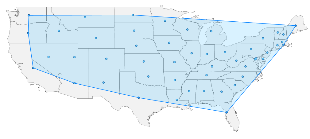
Jared produced a convex hull and minimum bounding circle with GeoScript Groovy in a recent post. I tried to replicate this workflow but quickly realized certain classes and functions weren’t available in GeoScript Python. Did it matter? Not very much in this case. Here’s the convex hull and minimum bounding circle for a shapefile of Washington weather stations produced in a previous post. Pay attention to what’s being imported.

from geoscript.layer import Shapefile
from geoscript.viewer import plot
from com.vividsolutions.jts.geom import GeometryCollection
from com.vividsolutions.jts.geom import GeometryFactory
from com.vividsolutions.jts.geom import PrecisionModel
from com.vividsolutions.jts.algorithm import MinimumBoundingCircle

#Get the point shapefile
staLayer = Shapefile('/home/gregcorradini/wa_stations.shp')

#Create a list of feature geometries
pntGeoms = [f.geom for f in staLayer.features()]

#Create a GeometryCollection from our list of points
geomColl = GeometryCollection(pntGeoms,GeometryFactory(PreciscionModel(),4326))

#Get the geometry collection's convex hull
geomConvexH = geomColl.convexHull()

#Get the geometry collection's minimum bounding circle
mCircle = (MinimumBoundingCircle(geomColl)).getCircle()

# Plot the geometries, BANG
plot(pntGeoms + [geomConvexH] + [mCircle])


I imported GeoScript modules and JTS Java classes in the example above. Jython can interoperate with Java libraries and classes because under the hood it’s Java. But how did I know what parameters a GeometryCollection accepted? I took a peek at the JTS Java doc and followed the bouncing argument ball. The weaving of colorful geometries happens after that thanks to the great plotting functionality from Justin.

There are tricks and trapdoors to this unwrapped exploration - the syntax is not as clean and intuitive as working with GeoScript Python. But a lot of magic still happens. I try to use functions that return geometry objects so I can plot them with the geoscript.viewer.plot function. This way I can see each step visually. Another advantage is that JTS and GeoTools have very well organized Java docs (here and there). It’s hard to fail at finding your way with road maps this good.

For example, mkgeomatics was deciding how to visually represent the output of a least-cost analysis he performed on a Bellingham, WA dataset. Part of the cartographic workflow used Voronoi diagrams that were built in ArcGIS. Both of us wondered if we could leverage GeoScript Python and JTS to solve the Voronoi diagram work. After a little sandbox scripting I came up with the following test code. It outlines how to derive a Voronoi diagram from a Delaunay triangulation (A more succinct way to build Voronoi diagrams would use the com.vividsolutions.jts.triangulate.VoronoiDiagramBuilder class. But Dr JTS produced an informative post on the relationship between both that I wanted to explore).
from geoscript.layer import Shapefile
from geoscript.viewer import plot
from com.vividsolutions.jts.geom import GeometryCollection
from com.vividsolutions.jts.geom import GeometryFactory
from com.vividsolutions.jts.geom import PrecisionModel
from com.vividsolutions.jts.algorithm import MinimumBoundingCircle
from com.vividsolutions.jts.triangulate import DelaunayTriangulationBuilder

#Get a point shapefile
staLayer = Shapefile('/home/gregcorradini/wa_stations.shp')

#Create a list of feature geometries
pntGeoms = [f.geom for f in staLayer.features()]

#Create a GeometryCollection from our list of points
geomColl = GeometryCollection(pntGeoms,GeometryFactory(PreciscionModel(),4326))

#Create a DelaunayTriangulationBuilder object and pass our geometry collection
dtb = DelaunayTriangulationBuilder()
dtb.setSites(geomColl)

#Get the Delaunay triangle faces
triangles = dtb.getTriangles(GeometryFactory(PrecisionModel(),4326))

#Make a pretty triangle picture
plot(pntGeoms + [triangles])


#Get the object's corresponding voronoi polygons in a java array
voronoiArray = dtb.getSubdivision().getVoronoiCellPolygons(GeometryFactory(PrecisionModel(),4326))

#Make a pretty picture
plot(pntGeoms + [i for i in voronoiArray])
That last Voronoi picture is hard to see in detail. So let's save off the Voronoi polygons to a shapefile and give each one the attributes of the original point that falls within it. The function 'changeGeometryType' is from a previous post.

#Create a voronoi geom.Poly schema based on old layer schema
voronoiSchema = changeGeometryType('voronoiWAStations',geom.Polygon,staLayer)

#Create voronoi layer
vLayer = ws.create(schema=voronoiSchema)

#For each voronoi polygon test which point is within it and pass attributes
for poly in voronoiArray:
for f in staLayer.features():

#Is my point within the polygon?
if f.geom.within(poly):

#Copy all point feature attributes into a dictionary
dictFeat = dict(f.iteritems())

#Overwrite the_geom with voronoi polygon
dictFeat['the_geom'] = poly

#Create a new feature and add it to voronoi layer
vLayer.add(voronoiSchema.feature(dictFeat))

The zoomed-in shot above shows the original points in pink, Delaunay triangles in gray and Voronoi diagram in green.

Tuesday, June 22, 2010

Geometry Plotting

I often have found myself looking for a quick and easy way to visualize a geometry object. Maybe I have a handful of geometry objects and I want to visualize some relationship (for example intersection) that exists between them.

Recently added to geoscript python is the ability to create an xy plot from a set of geometry objects. This functionality comes courtesy of the plot function that is located in the viewer module.


from geoscript.viewer import plot
from geoscript import geom

g = geom.LineString((0,0), (10,10))
plot(g)


Nothing all that earth shattering but something can be utilized in a variety of different ways. For instance visualizing an intersection as mentioned above:


g1 = geom.readWKT('POLYGON((-87.1875 49.5703125, -124.453125 -29.8828125, -92.8125 -58.7109375, -43.59375 -69.9609375, -4.21875 -60.1171875, 16.171875 -29.8828125, 16.171875 -5.2734375, 0 27.7734375, -20.390625 48.8671875, -55.546875 53.7890625, -78.046875 54.4921875, -87.1875 49.5703125))')

g2 = geom.readWKT('POLYGON((24.609375 51.6796875, -28.125 24.9609375, -25.3125 -20.7421875, 24.609375 -61.5234375, 74.53125 -51.6796875, 108.984375 -23.5546875, 92.109375 27.0703125, 61.171875 55.1953125, 40.078125 55.1953125, 24.609375 51.6796875))')

plot([g1.intersection(g2), g1,g2])


The plotting functionality makes use of the JFreeChart library, a popular open source Java framework for creating diagrams and charts. Another example of one of the benefits of the marriage of Java and Python that is Jython.

A recent use I made of this new functionality was with regard to geometry simplification. I wanted to quickly visualize a simplified geometry at different distance tolerances. Using everybody's favourite layer as an example:


from geoscript.layer import Shapefile
from geoscript.geom import simplify

shp = Shapefile('tests/work/states.shp')

texas = [f for f in shp.features("STATE_NAME = 'Texas'")][0].geom
plot(texas)

texas_simple = simplify(texas, 0.1)
plot(texas_simple)

texas_simple2 = simplify(texas, 0.5)
plot(texas_simple2)


The simplification routine is the Douglas-Peucker algorithm provided out of the box by JTS.

Sunday, June 20, 2010

Saving Weather Stations to a Shapefile with Python

The National Weather Service offers several XML data feeds related to weather conditions. In this tutorial we will use the list of all national observation stations to create a shapefile of Washington stations with Python.

def createXMLfileFromURL(strURL,strOutFilePath):

#Open url and read
res = urllib2.urlopen(strURL)
data = res.read()

#Write data to file
writer = open(strOutFilePath,'w')
writer.write(data)
writer.close()

if __name__=='__main__':

#Grab the XML feed and write it to a file
noaaIndexXML = '/home/gregcorradini/XMLfeeds/indexNOAAII.xml'
createXMLfileFromURL('http://www.weather.gov/xml/current_obs/index.XML',noaaIndexXML)

#Use ElementTree to walk XML for 'station'
root= (etree.parse(noaaIndexXML)).getroot()
listStations = root.findall('station')

#Findall WA stations in XML document
waStations = [i for i in listStations if i.findall('state')[0].text == 'WA']

#Create a dictionary for each station
dictWa = {}
for i in waStations:
#Notice we are using the lat/lng values to create a geom.Point
dictWa[i.findall('station_id')[0].text] = {'the_geom':geom.Point(float(i.findall('longitude')[0].text),float(i.findall('latitude')[0].text)),'station_id':i.findall('station_id')[0].text,'lat':float(i.findall('latitude')[0].text), 'lng':float(i.findall('longitude')[0].text), 'xml_url': i.findall('xml_url')[0].text}

#Create a schema for weather stations
staSchema = schema.Schema('wa_stations_notemp',[('the_geom',geom.Point,Projection('epsg:4326')),('station_id',str),('lat',float),('lng',float),('xml_url',str)])

#Get a workspace
ws = Directory('/home/gregcorradini/GeoTools/geoscript_wrk/isolines/data/US_shapefiles/')

#Create a stations shapefile with our schema
staLayer = ws.create('wa_stations_notemp',schema=staSchema)

#Create a feature for each station value
counter = 1
for key in dictWa.keys():
staFeature = staLayer.schema.feature(dictWa[key],str(counter))
staLayer.add(staFeature)
counter += counter

Tuesday, June 15, 2010

Merging Shapefiles with JavaScript

GeoScript aims to provide a framework for scripting common data processing tasks with GeoTools and the Java Topology Suite. Much in the same way that scripting languages like Python can leverage the powerful OGR/GDAL libraries, GeoScript offers similar functionality from languages that run on the JVM (currently Groovy, JavaScript, Python, or Scala).

In a recent post on his blog, Darren Cope wrote about merging a directory of shapefiles, a common data processing task. Here I'll demonstrate how to do the same thing with the JavaScript version of GeoScript.

This example uses the workspace and layer modules. I'm working with a directory containing shapefiles of US Census block groups for each state, merging them into a single shapefile for the country.


// import modules
var workspace = require("geoscript/workspace");
var layer = require("geoscript/layer");

// create workspaces from existing directories
var source = new workspace.Directory("path/to/source_dir");
var target = new workspace.Directory("path/to/target_dir");

// iterate through layers in source workspace
var country;
source.names.forEach(function(name) {
// create state layer from existing shapefile
var state = source.get(name);
// create country layer first time through
if (!country) {
country = new layer.Layer({
schema: state.schema.clone({name: "country"})
});
// this creates the new shapefile on disk
target.add(country);
}
// iterate through source features to add each to target
state.features.forEach(function(feature) {
country.add(feature);
});
});


While it is hard to beat the terseness of the ogr2ogr example, the JavaScript version of GeoScript provides syntax that I hope is familiar to a larger population of scripters.

Monday, June 14, 2010

Calculating Convex Hull and Minimum Bounding Circle with Groovy

The Java Topology Suite, which Groovy GeoScript wraps, contains spatial operators that act on a group of Features or Geometries. In this post, I collect all geometries from a shapefile to calculate the convex hull and minimum bounding circle. This post builds on previous blog entries where I use GeoScript to extract centroids and buffer Features.

Convex Hull
// Import GeoScript modules
import geoscript.layer.*
import geoscript.feature.*
import geoscript.geom.*

// Get the shapefile
Shapefile shp = new Shapefile('states_centroids.shp');

// Create a new Schema
Schema schema = new Schema('states_convex_hull', [['the_geom','Polygon','EPSG:4326']])

// Create our new Layer
Layer layer = shp.workspace.create(schema)

// Collect the Geometries
List geoms = shp.features.collect{f->f.geom}

// Create a GeometryCollection from the List of Geometries
GeometryCollection geomCol = new GeometryCollection(geoms)

// Get the Convex Hull from the GeometryCollection
Geometry convexHullGeom = geomCol.convexHull

// Add the Convex Hull Geometry as a Feature
layer.add(schema.feature([convexHullGeom]))


Minimum Bounding Circle

// Import GeoScript modules
import geoscript.layer.*
import geoscript.feature.*
import geoscript.geom.*

// Get the Shapefile
Shapefile shp = new Shapefile('states_centroids.shp')

// Create a new Schema
Schema schema = new Schema('states_minimum_bounding_circle', [['the_geom','Polygon','EPSG:4326']])

// Create the new Layer
Layer layer = shp.workspace.create(schema)

// Collect Geometries from the Shapefile
List geoms = shp.features.collect{f->f.geom}

// Create a GeometryCollection from the List of Geometries
GeometryCollection geomCol = new GeometryCollection(geoms)

// Get the Minimum Bounding Circle from the GeometryCollection
Geometry circleGeom = geomCol.minimumBoundingCircle

// Add the Minimum Bounding Circle Geometry as a Feature
layer.add(schema.feature([circleGeom]))

Saturday, June 12, 2010

Buffering Features with GeoScript Python

In a previous post, Jared buffered points and added them to a polygon shapefile. Here's the workflow in Python GeoScript.

from geoscript import proj
from geoscript import geom
from geoscript.layer import Shapefile
from geoscript.feature import schema

def changeGeometryType(strName,geomType,shpParent):

#Get all shapefile schema attributes except 'the_geom'
parentS = [(str(i.name),i.typ) for i in shpParent.schema.fields if not issubclass(i.typ,geom.Geometry)]

#Get shapefile Projection
pPrj = shpParent.schema.get('the_geom').proj

#Reinsert geomType into schema
parentS.insert(0,('the_geom',geomType,pPrj))

#Create centroid buffer schema
centroidSchema = schema.Schema(strName,parentS)

return centroidSchema


if __name__=='__main__':

#Get centroid shapefile
shp = Shapefile('/home/gregcorradini/GeoTools/geoscript_wrk/centroid_buffer/data/centroids.shp')

#Create a geom.Polygon schema from centroid schema
centroidSchema = changeGeometryType('centroid_buffer',geom.Polygon,shp)

#Get shapefile workspace
ws = shp.workspace

#Create a buffered centroid layer based on centroid schema
buffCentLayer = ws.create(schema=centroidSchema)

#For each centroid feature, create a buffered centroid, add it to buffered layer
for f in shp.features():

#Copy all feature attributes into a dictionary
dictFeat = dict(f.iteritems())

#Buffer 'the_geom' 3 degrees
dictFeat['the_geom'] = f.geom.buffer(3)

print dictFeat

#Create a buffered centroid feature with new dictionary attributes
buffFeature = buffCentLayer.schema.feature(dictFeat,f.id)

#Add new feature to buffered layer
buffCentLayer.add(buffFeature)


Calculating Centroids with GeoScript Python

Jared and Tim have shown us how to create centroids from a polygon shapefile in two different GeoScript implementations. Now let's see what the code looks like in Python GeoScript.

from geoscript import proj
from geoscript import geom
from geoscript.layer import Shapefile
from geoscript.feature import schema

def changeGeometryType(strName,geomType,shpParent):

#Put shapefile schema attributes except 'the geom' in a list of tuples
parentS = [(str(i.name),i.typ) for i in shpParent.schema.fields if not issubclass(i.typ,geom.Geometry)]

#Get shapefile Projection
pPrj = shpParent.schema.field('the_geom').proj

#reinsert geomType and proj into schema
parentS.insert(0,('the_geom',geomType,pPrj))

#create centroid schema with the list
centroidSchema = schema.Schema(strName,parentS)

return centroidSchema


if __name__=='__main__':

#Get states shapefile
shp = Shapefile('/home/gregcorradini/GeoTools/geoscript_wrk/centroid_buffer/data/US_shapefiles.shp')

#Substitute geom.Point into schema
centroidSchema = changeGeometryType('centroids',geom.Point,shp)

#Get workspace
ws = shp.workspace

#Create a centroid layer based on centroidSchema
centroidLayer = ws.create(schema=centroidSchema)

#Get all state features
stateFeatures = [f for f in shp.features()]

#For each state polygon get its centroid and add it to our centroid layer
for f in stateFeatures:

#create dictionary to hold each feature's attributes
newAtts = {}

for key in f.attributes.keys():
if issubclass(f.attributes[key].__class__,geom.Geometry):
newAtts[str(key)] = f.geom.centroid
else:
newAtts[str(key)] = f.attributes[key]

print newAtts

#Create a feature based on dictionary
centFeature = centroidLayer.schema.feature(newAtts,f.id)

#Add it to centroid layer
centroidLayer.add(centFeature)


Introducing GeoScript

GeoScript adds geo capabilities to dynamic scripting languages such as JavaScript, Python, Scala and Groovy.